
VNA time-domain reflection
A vector network analyzer (VNA) can locate a reflection without launching a physical pulse. It measures a circuit's complex response at a sequence of frequencies, preserving both amplitude and phase, then calculates what a chosen time-domain stimulus would produce. Keysight describes this as an inverse Fourier transform of frequency-domain measurements; its low-pass impulse and step displays are different transform choices. Keysight VNA time-domain documentation
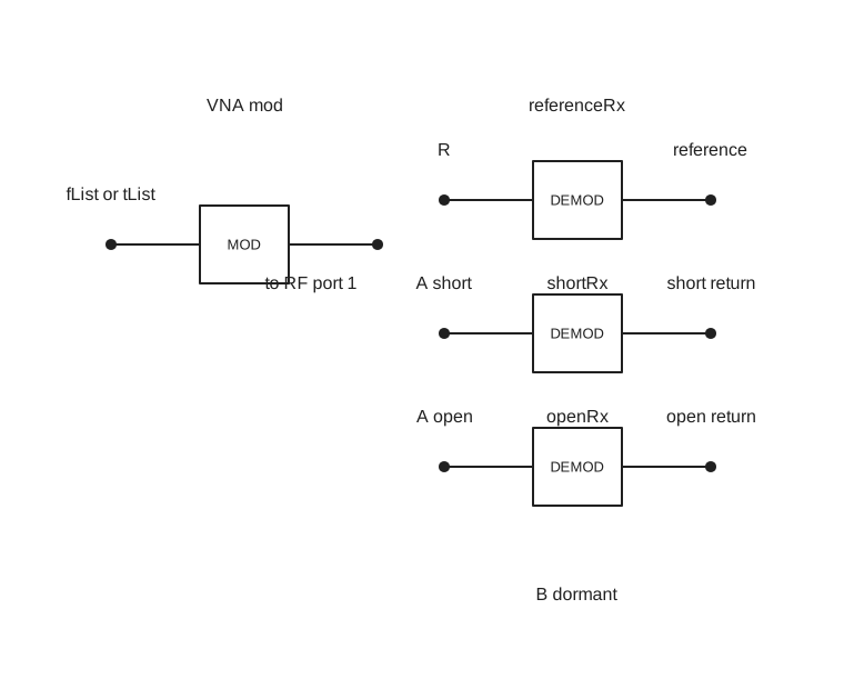
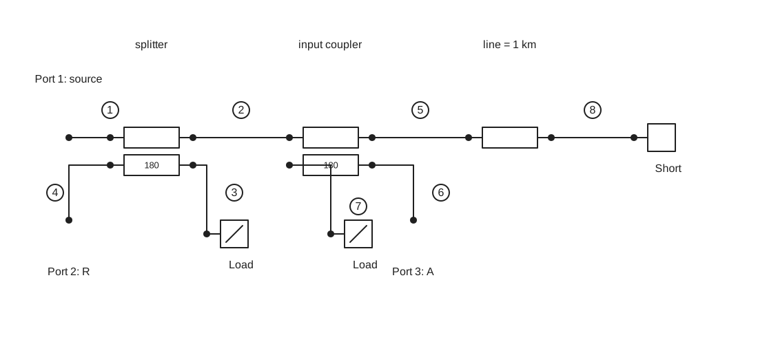
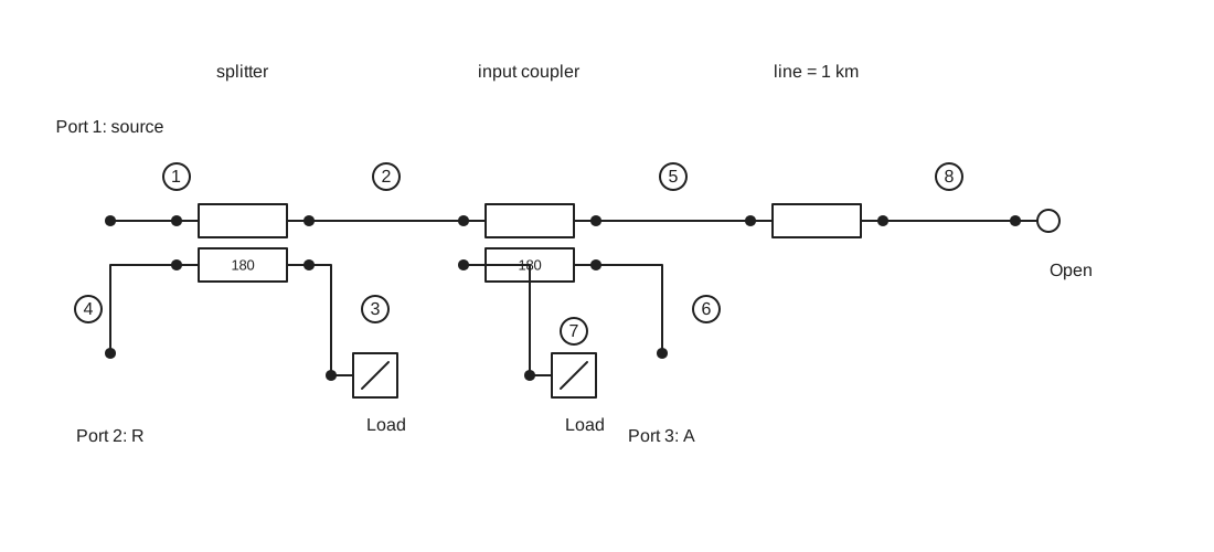
This note follows the VNA cable fault location REPL example. Both circuits use a matched splitter, an ideal input coupler, a matched 1 km lossless line, and a termination that is either a short or an open. Reference receiver R samples the source; reflection receiver A samples the return. The VNA's output coupler and receiver B remain dormant for this one-port test. The model produces a synthetic impulse response. It does not model an instrument sending a broadband pulse down the line.
Establish the frequency and time grids
The example asks for
Here
The complete record spans
For this grid,
The nonnegative frequency bins are
| Quantity | Value in the example | What it controls |
|---|---|---|
| Sample count | 4,096 | Number of reconstructed time samples |
| Sample rate | 250 MHz | 4 ns spacing between displayed samples |
| Frequency spacing | 61,035.15625 Hz | 16.384 µs unambiguous time period |
| Nonnegative bins | 2,049 | DC through Nyquist, including the zeroed Nyquist bin |
| Highest nonzero source bin | 124.93896484375 MHz | Finite synthesized bandwidth |
Build the synthetic pulse from cosine waves
nP.mod({mode: 'VNA-time'}) puts a real unit complex coefficient in each bin from DC through
With nP's inverse-transform convention, each full-spectrum bin contributes its coefficient divided by
Yes: it is a sum of equally spaced cosine waves, plus DC. The spacing is
The
At
With
If the Nyquist bin were also one, the samples would be a perfect periodic Kronecker impulse: 1 V at sample zero and 0 V at all other samples. nP instead zeros that bin. On the sample grid, the exact consequence is
Here
Let the RF circuit change each frequency
Each source bin passes through the circuit at its own frequency. Let
The zero-frequency transfer mod() populates global.fList, the n-port constructors calculate one S-parameter row per frequency, and demod(...).out('waveform') constructs the conjugate negative-frequency bins and calls the inverse FFT. nP evaluates DC directly in this ideal circuit. A physical RF VNA may extrapolate DC from measured low-frequency points; Keysight documents such extrapolation for its low-pass transforms. Keysight VNA time-domain documentation
The splitter sends a fraction
The one-way, matched Tlin(50, 1000) has phase factor
The A receiver uses referenceReceiver: referenceRx to divide by R and referenceGain: 2 to remove
Check the 2 km travel time
Tlin() uses nP's C0=299792458 m/s. This is the exact SI speed of light in vacuum. NIST CODATA speed of light
The termination is
For this model,
The predicted travel time is 6.671281904 µs, or 6671.281904 ns.
The REPL plots time in nanoseconds and displays a speed-of-light transit table calculated from the largest absolute sample in each return waveform. Sample 1668 is at
| Check | Short | Open |
|---|---|---|
| Predicted travel time | 6,671.282 ns | 6,671.282 ns |
| Time of plotted peak | 6,672 ns | 6,672 ns |
| Peak normalized response | −0.947616 | +0.947616 |
| Distance inferred from peak time | 1,000.108 m | 1,000.108 m |
| Peak-time difference from theory | +0.718 ns | +0.718 ns |
The time difference is smaller than one 4 ns sample interval. At the modeled velocity it corresponds to about 0.108 m of inferred one-way distance. The sample location agrees with the light-speed prediction; the small difference is expected when a continuous delay is read from a sampled, band-limited waveform. It does not indicate that the model uses a different propagation speed.
Why the short return briefly becomes positive
The short has a negative reflection coefficient, but its plotted return is not negative at every nearby time. The largest sample is −0.947616 at 6,672 ns; the next sample is +0.144052 at 6,676 ns. There is also a smaller positive sample of +0.093675 at 6,664 ns. These positive values are sidelobes of the same reflected impulse, not additional positive reflections or changes in the termination.
The normalized short-return waveform is the delayed, inverted synthetic impulse:
The finite, equally weighted cosine sum for
A frequency-domain taper could reduce the sidelobes, making a small nearby reflection easier to see. Its cost is a wider main pulse, so two close reflections become harder to separate. The current mod({mode: 'VNA-time'}) example uses equal bin weights and does not offer a window option. Keysight time-domain windowing
What the result does and does not represent
This is an ideal, lossless reference case. The chosen line has
The frequency interval sets the periodic time window, while the frequency span and any window applied to the bins set how sharply nearby reflections can be separated. Four-nanosecond displayed sample spacing is not, by itself, a claim of 4 ns physical resolution. This nP example uses equal bin weights, no tapering window, direct DC, and a zero Nyquist bin. It calculates an impulse-like response; it does not yet synthesize a step response or a user-selected pulse shape. For the sampling and transform foundations, see Sampling and quantization, FFT in nPort, and mod() in nPort.
Apply the same VNA to a two-port inductor
The VNA inductor impulse response example uses the same splitter and input coupler, inserts a 5 nH series inductor as the DUT, and activates the output coupler and receiver B. Its tList has 4,096 samples at 16 GHz. Consecutive times are 62.5 ps apart; the stored times run from 0 to 255.9375 ns, and the periodic record is 256 ns long. mod({mode: 'VNA-time'}) creates 2,049 nonnegative frequency bins from DC to the 8 GHz Nyquist frequency. Their spacing is 3.90625 MHz; the Nyquist source bin is zero.
The three plotted tables have different meanings:
| Receiver table | What is plotted |
|---|---|
R referenceRx.out('waveform') | The synthetic source impulse after the splitter, in volts. Its peak is about 0.707 V. |
A reflectionRx.out('waveform') | The inverse FFT of the inductor's normalized |
B transmissionRx.out('waveform') | The inverse FFT of the inductor's normalized |
A and B each divide their complex frequency bins by the gain-adjusted R receiver and use referenceGain: 2 to remove the two ideal coupler factors. The ratio is taken before the inverse FFT, so these two plots are dimensionless impulse responses. The R plot remains a receiver voltage. For the series inductor,
How to read the inductor plots
The 5 nH inductor is a series element. Its impedance is
The first two plotted samples make the behavior concrete:
| Time | R, reference voltage | A, normalized reflection | B, normalized transmission |
|---|---|---|---|
| 0 ps | +0.706934 V | +0.525463 | +0.474293 |
| 62.5 ps | +0.000173 V | −0.474638 | +0.474882 |
The A and B values add to the unit source impulse, about 0.999756 at time zero and 0.000244 at 62.5 ps. They do not add to R's voltage, because R includes the splitter's
The plots show a calculated response to a synthetic impulse, not a physical pulse launched by the VNA. Unlike the cable plot, there is no delayed return from a distant fault. If a feature appears close to 256 ns, it belongs to the inverse FFT's periodic time window; it is not a second reflection.
For a sweep that remains in the frequency domain and measures a 5 nH inductor's S11 and S21 with R, A, and B, see VNA frequency-domain measurement.