
What's new in nP 0.49.0
nP 0.49.0 brings circuit drawings, time-domain signals, and measurement experiments into the RF analysis workflow. Build a network, see its schematic, send a signal through it, and examine the result in time or frequency.
This page compares 0.49.0 with the published 0.0.48 release. The Obsidian plugin has its own release process in a separate repository.
Draw the network you analyze
Call nP.schematic(network) alongside your chart or table. nP reads the components and connections used to build the network, then draws an SVG using its bundled canonical symbols. You can draw a single component, a two-port cascade, an arbitrary nodal network, or a mod–circuit–demod signal path.
For a larger circuit, put familiar engineering arrangement names beside the connections. Here the intended drawing is a series section, a ladder, and another series section, all in one nodal network:
// Shape guidance beside the electrical connections
var g = nP.global;
g.fList = [2e9];

var r1 = nP.R(75);
var r2 = nP.R(50);
var c1 = nP.C(1e-12);
var tee1 = nP.Tee();
var short1 = nP.Short();

var network = nP.nodal(
    {series: [
        [r1, 1, 2],
        [r2, 2, 3]
    ]},
    {ladder: [
        [tee1, 4, 3, 5],
        [c1, 4, 6],
        [short1, 6],
        [r2, 5, 7]
    ]},
    {series: [
        [r1, 7, 8]
    ]},
    ['out', 1, 8]
);

nP.schematic(network);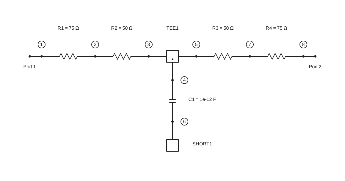
The numbered nodes come from the nodal() connection rows. Shape names guide the arrangement while the electrical connections remain authoritative. Reusing a component object, as this example does with r1 and r2, still creates separate drawing occurrences.
Supported shapes are series, ladder, bridgedT, branchline, edgeCoupledFilter, powerDivider, and powerCombiner. Without guidance, nP tries supported whole-network shape detection and then a generic layout. A flat netlist does not always reveal where an engineer intends one section to end and the next to begin; grouping supplies that missing information.
Live drawings include Copy as png and Fit drawing buttons, adjustable node/port/terminal dots, and a returned API exposing geometry, topology, detection, and errors. The pictures on this page are static SVG snapshots; open the REPL for the live controls.
Try grouped layouts and dot options · Try automatic shape detection · Read the Schematics guide
A time grid alongside the frequency grid
nP.global.tList holds sample times in seconds, just as fList holds analysis frequencies in hertz. tGen(start, stop, points) creates uniformly spaced times including both endpoints. This makes the sample interval, sample rate, and observation window explicit.
For 256 samples covering one 1 ms period without repeating its endpoint, use tGen(0, period * 255 / 256, 256). The sample interval is 3.90625 µs, the sample rate is 256 kHz, and the FFT bin spacing is 1 kHz. A time grid gives the FFT enough information to label its frequency axis in hertz.
The time grid connects several new operations:
| Operation | What the engineer supplies | What it provides |
|---|---|---|
waveform() | Shape, voltage levels, period, and a time grid | Sampled values and chart tables |
FFT() | Sample values and the matching uniform tList | Complex frequency bins, a populated fList, and output tables |
invFFT() | The complete complex spectrum | Reconstructed complex samples and time-domain tables |
Sampled mod() modes | Bits, text, or a PN source, rates, and matching tList | A transmitter with an analysis frequency grid |
demod() | The transmitter or signal-bearing RF network | Recovered waveforms, data, and measurement results |
Separate circuits can keep independent settings with nP.global(). Existing property access such as nP.global.fList = ... remains supported.
Read Global settings · Understand sampling and quantization
Waveform → FFT → inverse FFT
Create a square wave, triangle, full-wave rectified sine, or a custom piecewise-linear waveform. The following custom trapezoid is sampled, transformed to frequency bins, and reconstructed. Each stage produces its own table for lineChart(); the example needs no JavaScript mapping helper.
// Trapezoid in time, frequency, and reconstructed time
var g = nP.global;
var period = 1e-3;
g.tList = g.tGen(0, period * 255 / 256, 256);
g.fList = [];

var trapezoid = nP.waveform({
    shape: 'custom',
    period: period,
    points: [
        [0, 0],
        [0.1e-3, 1],
        [0.6e-3, 1],
        [0.7e-3, 0],
        [period, 0]
    ]
});

var samples = trapezoid.out('samples');
var fft = nP.FFT(samples);
var reconstructed = nP.invFFT(fft);

var timeTable = trapezoid.out('waveform');
var frequencyTable = fft.out('dBV');
var reconstructedTable = reconstructed.out('real');

nP.lineChart({
    inputTable: [timeTable],
    title: 'Sampled trapezoid',
    metricPrefix: 'milli',
    xAxisTitle: 'Time (ms)',
    yAxisTitle: 'Voltage (V)',
    showPoints: false
});
nP.lineChart({
    inputTable: [frequencyTable],
    title: 'Trapezoid FFT',
    plotType: 'bar',
    barBaseline: -80,
    yRange: [-80, 10],
    metricPrefix: 'kilo',
    xAxisTitle: 'Frequency (kHz)',
    yAxisTitle: 'Amplitude (dBV)'
});
nP.lineChart({
    inputTable: [reconstructedTable],
    title: 'Reconstructed trapezoid samples',
    metricPrefix: 'milli',
    xAxisTitle: 'Time (ms)',
    yAxisTitle: 'Voltage (V)',
    showPoints: false
});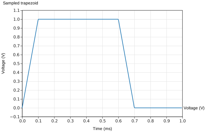
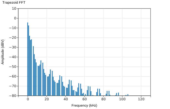
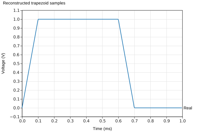
The reconstructed samples agree with the original samples to numerical precision. fft.out('dBV') supplies a one-sided RMS voltage spectrum for real voltage inputs, with a default display floor of −80 dBV. The complete complex fft array retains phase for reconstruction; the displayed dBV table is for plotting. FFT and inverse FFT also accept complex samples for other analyses.
Run the trapezoid round trip · See square-wave harmonics · See rectified-sine harmonics · Read FFT theory and nP usage
Send digital and modulated signals through RF networks
The new digital APIs make an RF network part of a signal experiment. mod() creates a transmitter, a cascade or nodal network carries its signal, and demod() reconstructs the receiver output. PN() produces clocked pseudorandom patterns; bitErrorRate() compares transmitted and received bits.
Examples range from sending ASCII text through an attenuator to PSK, QAM, and OFDM reception. Sampled carrier modes also include OOK, ASK, FSK, DPSK, QPSK, MSK, and GMSK. Analog AM, FM, PM, SSB, and DSB-SC modes support tone-based analysis.
Set the time grid before the transmitter, then create the RF components after mod() establishes their analysis frequencies. Receiver noise is enabled by default for sampled digital modes; turn it off for an ideal repeatable comparison. See the Guide for mode-specific sample counts, rates, and receiver settings.
Send ASCII through a circuit · Try QAM and OFDM · Compare bit error rates · Read Digital signals
Build a VNA experiment in frequency or time
Use the same reference, reflection, and transmission receiver approach for two different views of a DUT:
VNA-frequencyuses the selected frequency list to measure complex reflection and transmission. The inductor example compares receiver-derived S11 and S21 with the direct S-parameters ofnP.L(5e-9).VNA-timeuses a time grid to establish evenly spaced tones, applies the circuit response to those tones, and synthesizes an impulse response. The cable example shows opposite-polarity returns from open and short faults at 1 km.
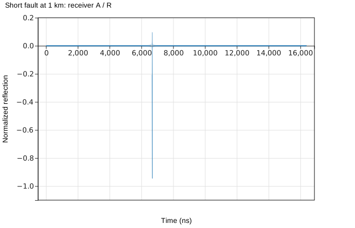
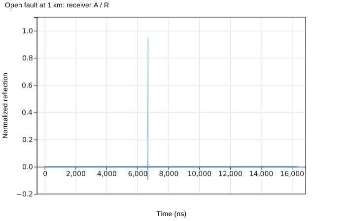
For this ideal line, the return travels 2 km at the speed of light: about 6.671 µs. The example includes a measured-versus-calculated transit-time table. Finite measurement bandwidth gives the synthesized pulse sidelobes; the Tech Note explains why a short's negative return can have a small positive excursion nearby.
Locate the cable fault · Measure inductor S-parameters · View its impulse response · Read the time-domain and frequency-domain VNA notes
Follow gain, noise, and distortion together
Noise and weak nonlinear source information now travel with connected n-ports. Amp() and Attn() make it straightforward to compare amplifier–attenuator ordering, including gain, noise figure, and output noise density. Two-tone analysis adds IM2, IM3, harmonics, and output intercept estimates through .out(...) selectors.
These models describe noise and weak-signal distortion under their documented conditions. They do not turn the network analysis into a general large-signal transient or compression simulator.
Compare amplifier and attenuator ordering · Plot two-tone IM3 · Read Noise and Intermodulation
More RF components and clearer examples
New constructors include Amp(), Attn(), Thru(), the ideal broadband Coupler180(), and the center-tapped three-port autotransformer trfAuto(). The 1N4148 model now connects DC bias inspection with RF, noise, and weak-signal distortion behavior. Matrix inversion and solving return new matrices without altering caller-owned data.
The Guide and REPL now share circuit examples with links between the explanation and the runnable code. Four separate low-pass examples show .cas(), cascade(), nodal(), and lpfGen() directly. Circuit illustrations are SVG output from the actual nP schematic and chart calls. Charts support bar plots, linear y-axis padding, and readable REPL output on narrow screens through horizontal scrolling.
Browse circuit examples · Explore RF constructors · Learn from engineering Tech Notes
Before updating
The version is 0.49.0, following 0.0.48. Ordinary global.fList access, flat nodal connection rows, cascades, and the existing combined RLC constructors remain available. The new time and signal APIs require attention to sample-grid and frequency-grid ordering. Shape groups help larger compositions; automatic detection cannot yet infer every intended section boundary.
See the release notes and compatibility checklist before migrating. An installed Obsidian plugin keeps its own pinned nP bundle until that separately maintained plugin is updated and released.