
Circuit examples
These circuits show how individual n-ports become useful RF networks. Each example sets its frequencies, creates its parts, connects them, then displays selected S-parameters. The code assumes the nP browser bundle has been loaded, as in Hello, nPort!.
The illustrations below are generated by running these code blocks with the current browser bundle. Each example calls nP.schematic() to draw its network; the accompanying chart or table comes from the same calculation.
Wilkinson power divider
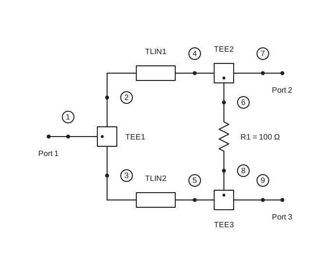
An ideal three-port junction splits the input into two quarter-wave branches. A 100 Ω resistor connects the output arms for isolation. The external port order is input, output 1, output 2.
// Wilkinson power divider

nP.global.fList = nP.global.fGen(4e9, 8e9, 41);

var inputTee = nP.Tee();
var outputTee1 = nP.Tee();
var outputTee2 = nP.Tee();
var branch1 = nP.Tlin(70.7, 0.49 * 0.0254);
var branch2 = nP.Tlin(70.7, 0.49 * 0.0254);
var isolationR = nP.R(100);

var divider = nP.nodal(
    [inputTee, 1, 2, 3],
    [branch1, 2, 4],
    [branch2, 3, 5],
    [outputTee1, 6, 4, 7],
    [outputTee2, 8, 5, 9],
    [isolationR, 6, 8],
    ['out', 1, 7, 9]
);

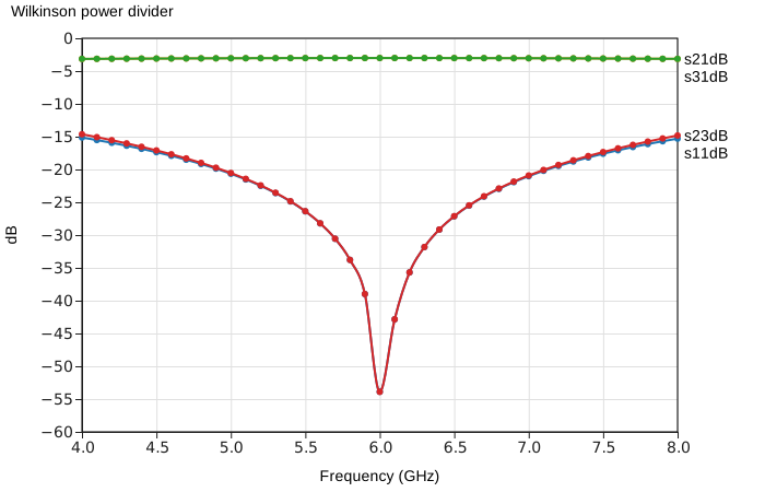
var response = divider.out('s11dB', 's21dB', 's31dB', 's23dB');
nP.schematic(divider);
nP.lineChart({
    inputTable: [response],
    title: 'Wilkinson power divider',
    metricPrefix: 'giga',
    xAxisTitle: 'Frequency (GHz)'
});
s21dB and s31dB show the two output paths. s11dB shows input match; s23dB shows isolation between the outputs. The line length above is close to a quarter wavelength near 6 GHz in the ideal vacuum-speed model.
Low-pass filter four ways
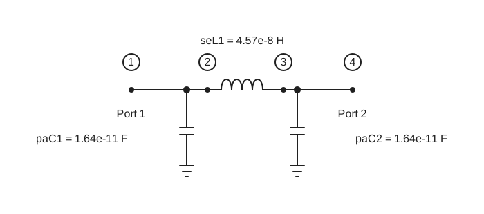
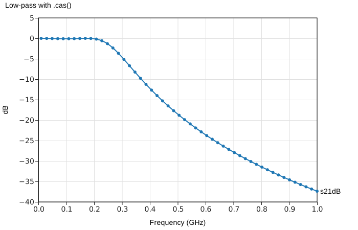
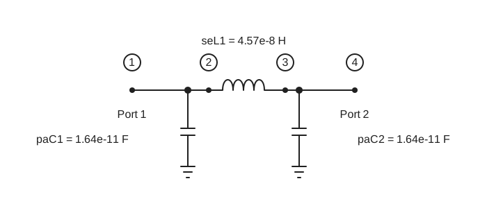
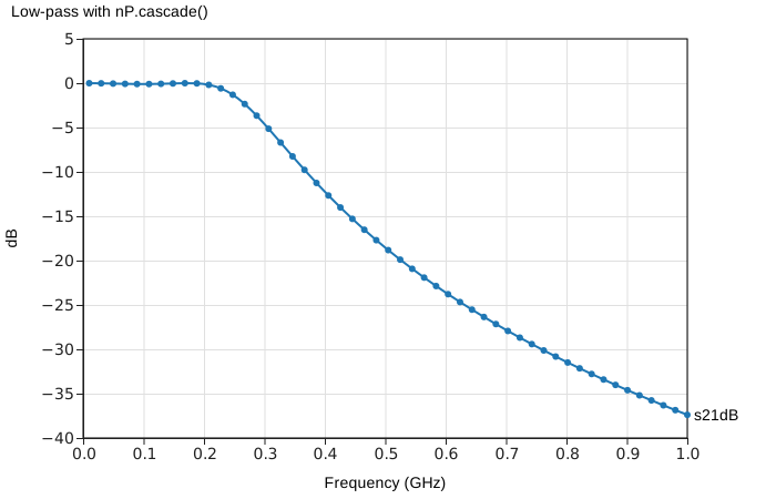
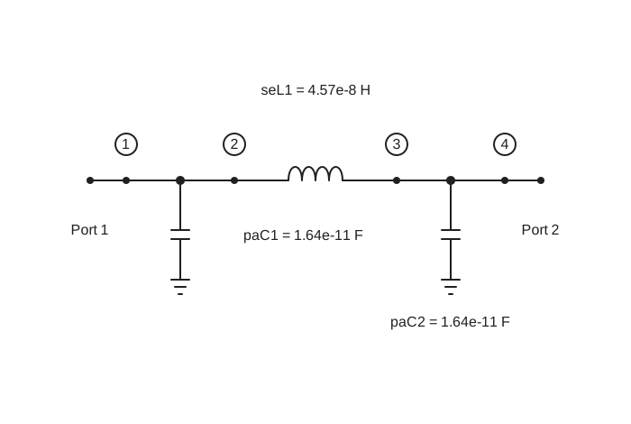
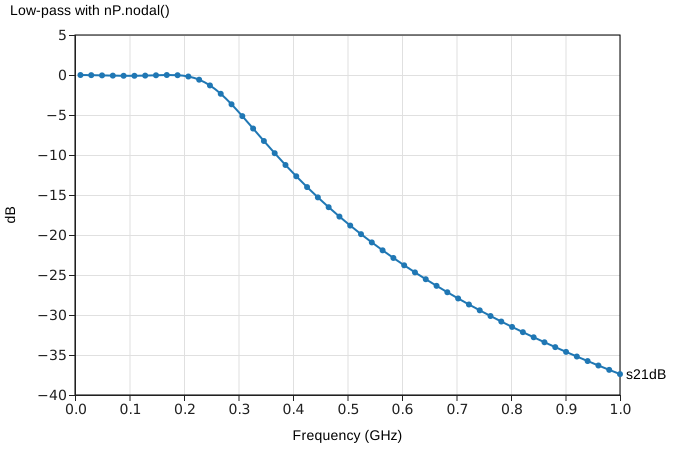
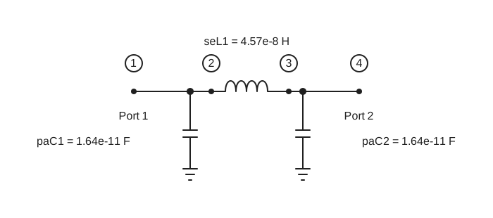
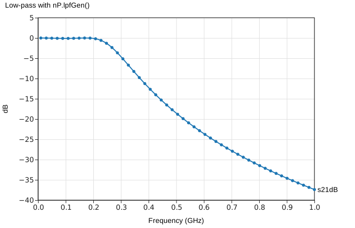
Here is the same three-element C-L-C filter connected four ways. Each example stands on its own and shows its own schematic and transmission response. The responses are the same.
The paC() parts include their shunt capacitors; seL() supplies the series inductor. See Filters for the Chebyshev helpers and a custom lpfGen() input.
Low-pass with .cas()
// Low-pass with .cas()

nP.global.fList = nP.global.fGen(10e6, 1e9, 51);

var c1 = nP.paC(16.41818746502858e-12);
var l1 = nP.seL(45.65360855435164e-9);
var c2 = nP.paC(16.41818746502858e-12);

var byMethod = c1.cas(l1).cas(c2);

var response = byMethod.out('s21dB');
nP.schematic(byMethod);
nP.lineChart({
    inputTable: [response],
    title: 'Low-pass with .cas()',
    metricPrefix: 'giga',
    xAxisTitle: 'Frequency (GHz)'
});
Low-pass with nP.cascade()
// Low-pass with nP.cascade()

nP.global.fList = nP.global.fGen(10e6, 1e9, 51);

var c1 = nP.paC(16.41818746502858e-12);
var l1 = nP.seL(45.65360855435164e-9);
var c2 = nP.paC(16.41818746502858e-12);

var byCascade = nP.cascade(c1, l1, c2);

var response = byCascade.out('s21dB');
nP.schematic(byCascade);
nP.lineChart({
    inputTable: [response],
    title: 'Low-pass with nP.cascade()',
    metricPrefix: 'giga',
    xAxisTitle: 'Frequency (GHz)'
});
Low-pass with nP.nodal()
// Low-pass with nP.nodal()

nP.global.fList = nP.global.fGen(10e6, 1e9, 51);

var c1 = nP.paC(16.41818746502858e-12);
var l1 = nP.seL(45.65360855435164e-9);
var c2 = nP.paC(16.41818746502858e-12);

var byNodes = nP.nodal(
    [c1, 1, 2],
    [l1, 2, 3],
    [c2, 3, 4],
    ['out', 1, 4]
);

var response = byNodes.out('s21dB');
nP.schematic(byNodes);
nP.lineChart({
    inputTable: [response],
    title: 'Low-pass with nP.nodal()',
    metricPrefix: 'giga',
    xAxisTitle: 'Frequency (GHz)'
});
Low-pass with nP.lpfGen()
// Low-pass with nP.lpfGen()

nP.global.fList = nP.global.fGen(10e6, 1e9, 51);

var byGenerator = nP.lpfGen([
    50,
    16.41818746502858e-12,
    45.65360855435164e-9,
    16.41818746502858e-12,
    50
]);

var response = byGenerator.out('s21dB');
nP.schematic(byGenerator);
nP.lineChart({
    inputTable: [response],
    title: 'Low-pass with nP.lpfGen()',
    metricPrefix: 'giga',
    xAxisTitle: 'Frequency (GHz)'
});
Pi attenuator
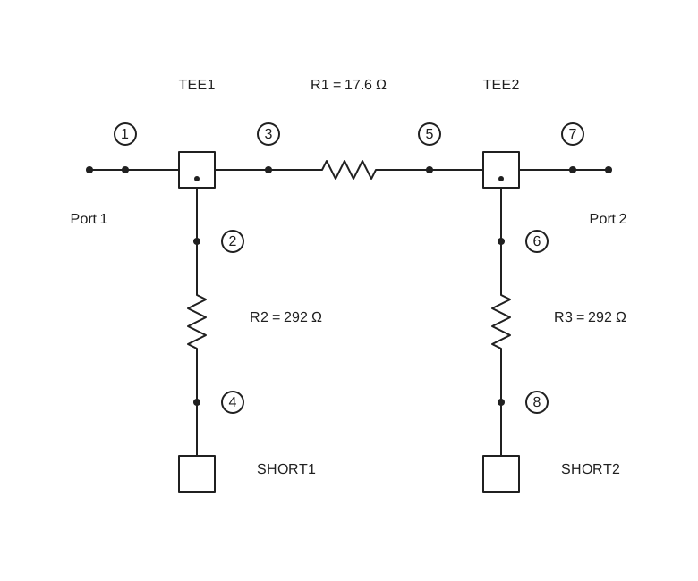
Two shunt resistors surround a series resistor. Each shunt path goes from Tee() port 1 through a resistor to Short(); the series resistor joins the two through paths.
// Pi attenuator

nP.global.fList = [2e9];

var inputShunt = nP.R(292.4);
var seriesR = nP.R(17.6);
var outputShunt = nP.R(292.4);
var inputTee = nP.Tee();
var outputTee = nP.Tee();
var ground = nP.Short();

var attenuator = nP.nodal(
    [inputTee, 2, 1, 3],
    [inputShunt, 2, 4],
    [ground, 4],
    [seriesR, 3, 5],
    [outputTee, 6, 5, 7],
    [outputShunt, 6, 8],
    [ground, 8],
    ['out', 1, 7]
);

var response = attenuator.out('s11dB', 's21dB');
nP.schematic(attenuator);
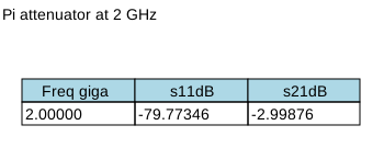
nP.lineTable({
    inputTable: [response],
    title: 'Pi attenuator at 2 GHz'
});
This illustrates how a circuit of three separate resistors can be measured as a single two-port. The Connecting nPorts page explains the connection labels.
Edge-coupled bandpass filter
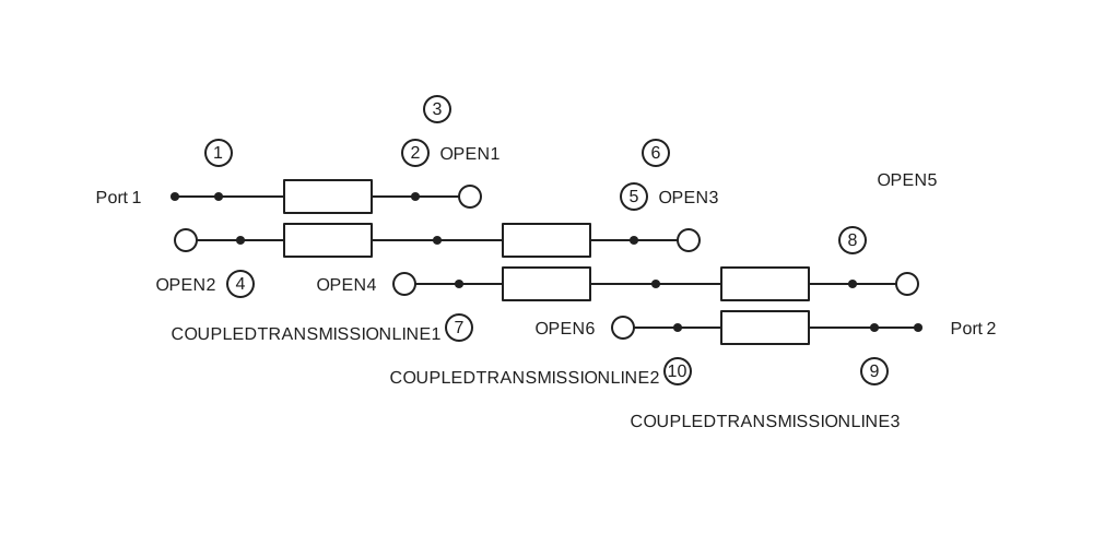
Three ideal coupled-line sections form this filter. Tclin() ports are numbered clockwise from the upper left. The unused ends are terminated with Open() fixtures.
// Edge-coupled bandpass filter

nP.global.fList = nP.global.fGen(4e9, 8e9, 21);

var coupled1 = nP.Tclin(79.667, 37.834, 0.491 * 0.0254);
var coupled2 = nP.Tclin(60.866, 42.505, 0.491 * 0.0254);
var coupled3 = nP.Tclin(79.667, 37.834, 0.491 * 0.0254);
var open = nP.Open();

var filter = nP.nodal(
    [coupled1, 1, 2, 3, 4],
    [coupled2, 3, 5, 6, 7],
    [coupled3, 6, 8, 9, 10],
    [open, 2],
    [open, 4],
    [open, 5],
    [open, 7],
    [open, 8],
    [open, 10],
    ['out', 1, 9]
);

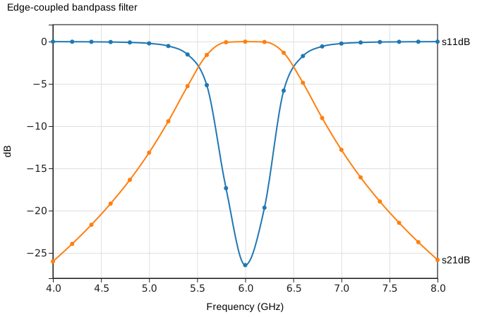
var response = filter.out('s11dB', 's21dB');
nP.schematic(filter);
nP.lineChart({
    inputTable: [response],
    title: 'Edge-coupled bandpass filter',
    metricPrefix: 'giga',
    xAxisTitle: 'Frequency (GHz)'
});
For the coupled-line port order and defaults, see Ideal components.