
Digital signals
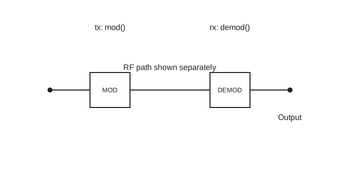
Use nP.mod() to make a signal, send it through an n-port circuit, and use nP.demod() to recover the output. nP.PN() makes a clocked pseudorandom bit pattern when you need control over the clock ticks. nP.bitErrorRate() measures the fraction of received bits in error.
Sample a periodic waveform
nP.global.tList holds sample times in seconds, much as fList holds analysis frequencies. nP.waveform() uses that time list by default, or accepts a time list of its own. It returns sampled voltages without changing either global list.
var g = nP.global;
var period = 1e-3;
g.tList = g.tGen(0, period * 255 / 256, 256);

var triangle = nP.waveform({
    shape: 'triangle',
    period: period
});

var triangleTable = triangle.out('waveform');
nP.lineChart({
    inputTable: [triangleTable],
    title: 'Triangle wave',
    metricPrefix: 'milli',
    xAxisTitle: 'Time (ms)',
    yAxisTitle: 'Voltage (V)'
});
The triangle defaults to a symmetric rise (riseFraction: 0.5) between −1 V and +1 V. Set lowVolts and highVolts for other levels. For an ideal square wave, use nP.waveform({shape: 'square', period: period}); it defaults to a 50% duty cycle and the same voltage levels. Set dutyCycle to change the high-state fraction. For a full-wave rectified sine, use nP.waveform({shape: 'rectifiedSine', period: period}). It ranges from 0 V to 1 V by default; period describes the original sine, and the output repeats every half period. Its spectrum contains DC and even multiples of the original sine frequency. For a custom periodic shape, set shape: 'custom' and pass points: [[0, lowVoltage], [peakTime, peakVoltage], [period, lowVoltage]]; waveform() linearly interpolates between those points. out('samples') returns an array suitable for nP.FFT(), and out('time') returns the sampling times. The chart table uses seconds, so metricPrefix: 'milli' displays milliseconds. When taking an FFT of one period, omit the duplicate sample at exactly one period. mod({input: ...}) currently accepts PN waveforms only.
nP.FFT() transforms a sampled waveform into complex frequency bins and fills global.fList. Its .out('dBV') method returns a chart-ready, one-sided RMS voltage spectrum from DC through Nyquist, with values below −80 dBV displayed at that floor.
var g = nP.global;
var period = 1e-3;
g.tList = g.tGen(0, period * 255 / 256, 256);
g.fList = [];

var rectified = nP.waveform({
    shape: 'rectifiedSine',
    period: period
});
var rectifiedSamples = rectified.out('samples');
var fft = nP.FFT(rectifiedSamples);
var harmonics = fft.out('dBV');

nP.lineChart({
    inputTable: [harmonics],
    plotType: 'bar',
    barBaseline: -80,
    yRange: [-80, 10],
    metricPrefix: 'kilo',
    xAxisTitle: 'Frequency (kHz)',
    yAxisTitle: 'Amplitude (dBV)'
});
The fft array retains the complex FFT bins. Use fft.out('dBV', {floorDbv: -100}) to change the display floor. The table includes DC and every nonnegative bin through Nyquist; the rectified sine has its strongest AC terms at even multiples of the original 1 kHz frequency.
Send text through a circuit
var circuit = nP.global();
circuit.tList = circuit.tGen(0, 831 / 8e9, 832); // 13 ASCII characters × 8 bits × 8 samples.
circuit.fList = [];

var tx = nP.mod({
    mode: 'ASCII',
    message: 'Hello, nPort!'
});

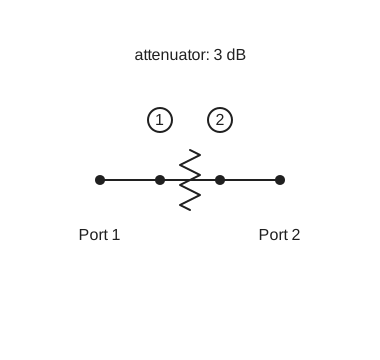
var attenuator = nP.Attn(3);
var chain = nP.cascade(attenuator, {signal: tx});
var rx = nP.demod(chain, {noise: false});

var receivedText = rx.out('ASCII text');
var receivedWaveform = rx.out('waveform');
nP.log(receivedText);
nP.lineChart({
    inputTable: [receivedWaveform],
    title: 'Received waveform',
    metricPrefix: 'none',
    xAxisTitle: 'Time (ns)',
    yAxisTitle: 'Voltage (V)'
});
For this sampled digital mode, mod() requires one uniformly spaced tList entry per generated sample and fills the selected circuit's frequency list with the signal's FFT frequencies. Create the attenuator after mod() so its S-parameter rows use those frequencies. {signal: tx} attaches the transmitter to the circuit. demod() normally includes receiver noise for sampled digital modes; {noise: false} makes this first example repeatable. The waveform table's time values are already in nanoseconds, so the chart uses metricPrefix: 'none'.
Make a transmitter with mod()
With no options after selecting a 1,016-point time grid, nP.mod() makes one period of PN7 bits at 1 Gbit/s, with 8 samples per bit, 0 V for zero, and 1 V for one. The carrier defaults to 0 Hz, giving a baseband signal. The resulting object describes a signal; it is not itself an n-port.
var g = nP.global;
g.tList = g.tGen(0, 1015 / 8e9, 1016);
g.fList = [];
var tx = nP.mod(); // PN7 baseband, 127 bits
g.tList = g.tGen(0, 1023 / 640e6, 1024);
g.fList = [];
var textTx = nP.mod({
    mode: 'ASCII',
    message: 'Hi',
    bitRate: 10e6,
    samplesPerBit: 64
});
g.tList = g.tGen(0, 31 / 8e9, 32);
g.fList = [];
var bitTx = nP.mod({mode: 'bits', bits: '0101'});
Use mode: 'ASCII' with a nonempty seven-bit ASCII message, mode: 'bits' with a nonempty 0/1 string or array, or mode: 'PN2' through 'PN16' for a repeating pseudorandom sequence. Set bitRate, samplesPerBit, lowVolts, and highVolts in the options object as needed. An RF carrier must remain below the sample Nyquist frequency; increase samplesPerBit when raising carrierHz.
To put bits on an RF carrier, select a modulation mode and provide a positive carrierHz:
var g = nP.global;
g.tList = g.tGen(0, 1023 / 640e6, 1024);
g.fList = [];
var tx = nP.mod({
    mode: 'PSK',
    message: 'Hi',
    carrierHz: 200e6,
    bitRate: 10e6,
    samplesPerBit: 64
});| Mode | Signal |
|---|---|
OOK | Carrier on for 1, off for 0; default levels 0 V and 1 V. |
ASK | Two nonzero carrier levels; default levels 0.5 V and 1 V. |
FSK | Two carrier frequencies; default deviation is half the bit rate. |
PSK, DPSK | Binary phase and differential phase modulation. PSK uses NRZ encoding by default; it also supports encoding: 'Manchester'. |
QPSK, QAM | I/Q symbols. QAM defaults to 16 points and supports orders 4, 16, 64, and 256. |
MSK, GMSK | Continuous-phase modulation; GMSK defaults to bt: 0.3. |
OFDM | Multicarrier modulation using symbolRate and fftSize. |
For these RF modes, message or bits chooses the data automatically; otherwise the data defaults to PN7. You can set dataMode explicitly to 'ASCII', 'bits', or a PN mode. mod() also supports the analog modes AM, FM, PM, SSB, and DSB-SC; those modes create tone-based analyses rather than sampled digital bit streams. They still require a valid selected tList, although their sparse tone frequencies do not depend on its spacing.
Inspect the transmitter
tx.out('waveform') returns a chart-ready table with Time (ns) and Output (V) columns. Other useful selectors are:
| Selector | Result |
|---|---|
'settings' | Mode, rates, levels, carrier, sample count, and other applicable settings. |
'mode' | Selected mode name. |
'bit count', 'sample count', 'frequency count' | Counts. |
'frequencies' | FFT frequencies in hertz. |
'frequency table' | Table of FFT bin numbers and frequencies. |
'spectrum' | Array of complex FFT values. |
For bit modes, tx.bits contains the transmitted bits. For separate circuits, create a new context with nP.global() before each mod() call; its frequency list can start empty. If you pass fftList: someArray, mod() fills that array instead of the selected context's fList.
Make a clocked PN pattern
nP.PN() defaults to 7 stages, an all-ones seed, and 0 V / 1 V output. It uses nP.global.tList unless you supply time. Each time entry is one clock tick. The time list must increase uniformly and contain a whole number of PN periods; a period has 2 ** stages - 1 ticks.
var circuit = nP.global();
circuit.tList = circuit.tGen(0, 6e-9, 7); // PN3: seven 1 ns ticks

var pn = nP.PN({stages: 3});
var pnWaveform = pn.out('waveform');
nP.lineChart({
    inputTable: [pnWaveform],
    title: 'PN3 clocked waveform',
    metricPrefix: 'none',
    xAxisTitle: 'Time (ns)',
    yAxisTitle: 'Voltage (V)'
});pn.out('bits'), out('samples'), and out('time') return arrays. out('bit string') returns the bits as consecutive 0 and 1 characters. out('waveform') returns a chart table; out('bit count'), out('sample count'), out('bit rate'), out('sample rate'), and out('clock rate') return counts or rates. To send this exact clocked pattern through a circuit, first replace the selected tList with the complete sample grid, then use nP.mod({input: pn}) before constructing the n-port components. Modulation expands each PN clock tick to 8 samples by default; set samplesPerBit to change that density and update tList accordingly.
Recover a signal with demod()
nP.demod(chain) reads the signal attached to the completed n-port. For a quick ideal connection, nP.demod(tx) accepts a transmitter directly. Receiver noise is on by default for sampled digital signals; each demod() call draws a new noise waveform. Outputs read from one rx object use the same draw.
var rx = nP.demod(chain, {
    noise: false,
    outputPort: 2
});

var receivedText = rx.out('ASCII text');
var receivedBits = rx.out('bits');
nP.log(receivedText);
nP.log(receivedBits);
The output port defaults to 2, and the input port defaults to 1. Set outputPort or inputPort for a different circuit port. thresholdVolts overrides the automatically estimated bit-decision threshold. rx.out('waveform') returns received voltage versus time in nanoseconds; out('bits') returns decided bits, out('bit string') returns those bits as consecutive characters, and out('ASCII text') decodes complete eight-bit bytes. Transmitters from mod() also support out('bit string'). Other useful outputs include 'bit count', 'sample count', 'frequency count', 'frequencies', and 'spectrum'. For carrier modes, 'carrier waveform' returns the received passband samples while 'waveform' returns the recovered levels. ASCII decoding has no clock recovery or error correction.
Measure bit error rate
nP.bitErrorRate(tx, chain) compares the known transmitted bits with 100 independent receptions by default and returns the error fraction from 0 to 1. Set receptions to change the number of trials. Receiver options such as noise, outputPort, and thresholdVolts can be passed in the same object.
// Bit error rate: create a matching transmitter and circuit together
var berContext = nP.global();
berContext.tList = berContext.tGen(0, 31 / 8e9, 32);
berContext.fList = [];

var berTx = nP.mod({mode: 'bits', bits: '1010'});
var berAttenuator = nP.Attn(3);
var berChain = nP.cascade(berAttenuator, {signal: berTx});
var ber = nP.bitErrorRate(berTx, berChain, {receptions: 100});
nP.log(ber);
This example creates its own analysis context, transmitter, and circuit, so it can run independently of the earlier examples. Each reception calls demod() again, so a noisy result can differ between runs. For a signal-only check, pass {noise: false}. The transmitter and circuit must carry the same bit pattern and frequency grid.
VNA cable fault location
A vector network analyzer measures the complex response at successive frequencies and calculates a time-domain impulse from those measurements. mode: 'VNA-time' models that calculation with a unit reference at each frequency bin, rather than transmitting a physical pulse. The frequency list runs from DC through Nyquist; the Nyquist reference is zero so the inverse transform remains real. The modeled circuit supplies its DC value directly, whereas a physical RF VNA commonly needs a low-frequency extrapolation. This mode requires a power-of-two tList beginning at zero, and has no bits or carrier.
var g = nP.global();
g.tList = g.tGen(0, 4095 / 250e6, 4096);
g.fList = [];

var tx = nP.mod({mode: 'VNA-time'});

var splitter = nP.Coupler180();
var inputCoupler = nP.Coupler180();
var line = nP.Tlin(50, 1000);
var short = nP.Short();
var open = nP.Open();
var load = nP.Load();

var shortCircuit = nP.nodal(
    [splitter, 1, 2, 3, 4],
    [inputCoupler, 2, 5, 6, 7],
    [line, 5, 8],
    [short, 8],
    [load, 3],
    [load, 7],
    ['out', 1, 4, 6],
    {signal: tx, inputPort: 1}
);

var openCircuit = nP.nodal(
    [splitter, 1, 2, 3, 4],
    [inputCoupler, 2, 5, 6, 7],
    [line, 5, 8],
    [open, 8],
    [load, 3],
    [load, 7],
    ['out', 1, 4, 6],
    {signal: tx, inputPort: 1}
);

var referenceRx = nP.demod(shortCircuit, {outputPort: 2, referenceGain: 1, noise: false});
var shortRx = nP.demod(shortCircuit, {outputPort: 3, referenceReceiver: referenceRx, referenceGain: 2, noise: false});
var openRx = nP.demod(openCircuit, {outputPort: 3, referenceReceiver: referenceRx, referenceGain: 2, noise: false});
var inputTable = referenceRx.out('waveform');
var shortReturn = shortRx.out('waveform');
var openReturn = openRx.out('waveform');

nP.lineChart({
    inputTable: [inputTable],
    title: 'VNA reference receiver R',
    xAxisTitle: 'Time (ns)',
    yAxisTitle: 'Voltage (V)',
    metricPrefix: 'none',
    showPoints: false
});

nP.lineChart({
    inputTable: [shortReturn],
    title: 'Short fault at 1 km: receiver A / R',
    xAxisTitle: 'Time (ns)',
    yAxisTitle: 'Normalized reflection',
    metricPrefix: 'none',
    showPoints: false
});

nP.lineChart({
    inputTable: [openReturn],
    title: 'Open fault at 1 km: receiver A / R',
    xAxisTitle: 'Time (ns)',
    yAxisTitle: 'Normalized reflection',
    metricPrefix: 'none',
    showPoints: false
});
The 4,096 time points give 2,049 nonnegative frequency bins, about 61 kHz apart, and a 16.384 µs unambiguous time window. The splitter feeds receiver R; the input coupler feeds reflection receiver A. The output coupler and B receiver are dormant for this one-port cable test. The short has reflection coefficient
For the pulse equation and a numerical check of the 2 km round-trip travel time, see VNA time-domain reflection.
VNA frequency-domain measurement
VNA-frequency sweeps the supplied fList with one unit complex reference at each frequency. It does not require tList, equally spaced frequencies, or an FFT. demod() reads a complex receiver phasor at each point. out('spectrum') contains raw voltage phasors. With referenceReceiver, out('response') divides the selected receiver by the reference receiver's gain-adjusted response at each frequency and applies the settable referenceGain. The gain defaults to unity, including for a direct connection. The response selectors also provide chart tables. Frequency-domain reception supports noise: false; noise simulation is not available in this mode.
In the VNA inductor S-parameters REPL example, an ideal splitter feeds reference receiver R and the input coupler. The input coupler samples reflection at A; the output coupler samples transmission at B. Each test path has half the voltage seen by R, times the inductor's S-parameter. Set R's gain to 1 and A/B gains to 2, with referenceReceiver: referenceRx for A and B. A changed reference path, such as a 3 dB pad, requires a corresponding gain adjustment.
var g = nP.global;
g.fList = g.fGen(1e9, 3e9, 101);

var tx = nP.mod({mode: 'VNA-frequency', fList: g.fList});
var splitter = nP.Coupler180();
var inputCoupler = nP.Coupler180();
var outputCoupler = nP.Coupler180();
var l1 = nP.L(5e-9);
var load = nP.Load();

var circuit = nP.nodal(
    [splitter, 1, 2, 3, 4],
    [inputCoupler, 2, 5, 6, 7],
    [l1, 5, 8],
    [outputCoupler, 8, 9, 10, 11],
    [load, 3],
    [load, 7],
    [load, 9],
    [load, 10],
    ['out', 1, 4, 6, 11],
    {signal: tx, inputPort: 1}
);

var referenceRx = nP.demod(circuit, {outputPort: 2, referenceGain: 1, noise: false});
var reflectionRx = nP.demod(circuit, {outputPort: 3, referenceReceiver: referenceRx, referenceGain: 2, noise: false});
var transmissionRx = nP.demod(circuit, {outputPort: 4, referenceReceiver: referenceRx, referenceGain: 2, noise: false});
var s11Table = reflectionRx.out('response dB');
var s21Table = transmissionRx.out('response dB');

nP.lineChart({inputTable: [s11Table], title: 'Inductor S11', metricPrefix: 'giga'});
nP.lineChart({inputTable: [s21Table], title: 'Inductor S21', metricPrefix: 'giga'});
The VNA frequency-domain measurement note derives the three receiver paths and the expected complex S11 and S21 values at 2 GHz. The VNA inductor impulse response example uses the same three-receiver circuit with VNA-time.